Axial extension in a homogeneous pipe
Section author: Jagir Hussan <https://unidirectory.auckland.ac.nz/profile/rjag008>, David Nickerson <http://about.me/david.nickerson/>
This example demonstrates the application of an mechanical extension to a homogeneous tissue cylinder model along the axis of the cylinder. The Mooney-Rivlin constitutive law is used via CellML.
This is a Python example. In order to exectute this example, you will need to have the OpenCMISS Python bindings available. This Cmgui command file can be used to visualise the simulation output. The geometric finite element mesh used in this example was created using PyZinc with the script quadcylinderthreematerials.py.
The example is encoded in HomogeneousPipeAxialExtension.py. Below we describe some of the key aspects of this example.
Example description
In this example the The Python script exfile.py is used to load the geometry from a file in the Zinc EX format.
1 2 3 | import sys, os, exfile
# Make sure $OPENCMISS_ROOT/cm/bindings/python is first in our PYTHONPATH.
sys.path.insert(1, os.path.join((os.environ['OPENCMISS_ROOT'],'cm','bindings','python')))
|
The exfile.py script in needs to be in the current folder or available in your Python environment for the import on line 1 to succeed. Whereas on line 3 we are specifically adding the location we expect to find the OpenCMISS Python bindings using the OPENCMISS_ROOT environment variable. Using the exfile module we are able to load the finite element model geometry from the EXREGION file: hetrogenouscylinder.exregion, as shown below:
1 2 | #Load the mesh information in the form of exregion format
exregion = exfile.Exregion("hetrogenouscylinder.exregion")
|
Throughout the remainder of the Python script you can see the data from the now defined exregion object used to create the geometric mesh via the standard OpenCMISS methods. For example, in this code:
1 2 3 4 5 6 7 8 9 10 11 12 13 14 15 16 17 18 19 20 21 | # Read the geometric field
for node_num in exregion.nodeids:
version = 1
derivative = 1
coord = []
for component in range(1, numberOfXi + 1):
component_name = ["1", "2", "3"][component - 1]
value = exregion.node_value("coordinates", component_name, node_num, derivative)
geometricField.ParameterSetUpdateNodeDP(
CMISS.FieldVariableTypes.U,
CMISS.FieldParameterSetTypes.VALUES,
version, derivative, node_num, component, value)
coord.append(value)
#The cylinder has an axial length of 5 units and coord[2] contains the axial coordinate value
if coord[2] < 0.001:
left_boundary_nodes.append(node_num)
elif coord[2] > 4.999:
right_boundary_nodes.append(node_num)
geometricField.ParameterSetUpdateFinish(CMISS.FieldVariableTypes.U,CMISS.FieldParameterSetTypes.VALUES)
|
we set the nodal coordinates and derivatives in the models geometric field. There is also code to keep track of nodes located at either end of the vessel, which will be used later when defining boundary conditions.
CellML
As mentioned above, this example uses the Mooney-Rivlin mechanical constitutive law defined in CellML. In this section we briefly describe how this is achieved, further details and general description can be found in the OpenCMISS CellML Examples. First the CellML environment must be created and our Mooney-Rivlin model imported into the environment:
1 2 3 4 5 | # Create the CellML environment
CellML = CMISS.CellML()
CellML.CreateStart(CellMLUserNumber, region)
# Import a Mooney-Rivlin material law from a file
MooneyRivlinModel = CellML.ModelImport("mooney_rivlin.xml")
|
With the CellML model imported, we are now able to flag the variables from the model that are known (by the finite elasticity model) and those variables that are wanted (by the finite elasticity model) from the CellML model. These are the variables from the CellML model that we will want to associate with fields in the OpenCMISS (continuum) model.
1 2 3 4 5 6 7 8 9 10 11 12 13 14 | # Now we have imported the model we are able to specify which variables from the model we want to set from openCMISS
CellML.VariableSetAsKnown(MooneyRivlinModel, "equations/E11")
CellML.VariableSetAsKnown(MooneyRivlinModel, "equations/E12")
CellML.VariableSetAsKnown(MooneyRivlinModel, "equations/E13")
CellML.VariableSetAsKnown(MooneyRivlinModel, "equations/E22")
CellML.VariableSetAsKnown(MooneyRivlinModel, "equations/E23")
CellML.VariableSetAsKnown(MooneyRivlinModel, "equations/E33")
# and variables to get from the CellML
CellML.VariableSetAsWanted(MooneyRivlinModel, "equations/Tdev11")
CellML.VariableSetAsWanted(MooneyRivlinModel, "equations/Tdev12")
CellML.VariableSetAsWanted(MooneyRivlinModel, "equations/Tdev13")
CellML.VariableSetAsWanted(MooneyRivlinModel, "equations/Tdev22")
CellML.VariableSetAsWanted(MooneyRivlinModel, "equations/Tdev23")
CellML.VariableSetAsWanted(MooneyRivlinModel, "equations/Tdev33")
|
Having flagged the variables we require from the CellML model, we can map them to fields, more specifically, the components of field variables. First we map the strain tensor from the finite elasticity model to variables in the CellML model:
1 2 3 4 5 6 7 | #Map the strain components
CellML.CreateFieldToCellMLMap(dependentField,CMISS.FieldVariableTypes.U1,1, CMISS.FieldParameterSetTypes.VALUES,MooneyRivlinModel,"equations/E11", CMISS.FieldParameterSetTypes.VALUES)
CellML.CreateFieldToCellMLMap(dependentField,CMISS.FieldVariableTypes.U1,2, CMISS.FieldParameterSetTypes.VALUES,MooneyRivlinModel,"equations/E12", CMISS.FieldParameterSetTypes.VALUES)
CellML.CreateFieldToCellMLMap(dependentField,CMISS.FieldVariableTypes.U1,3, CMISS.FieldParameterSetTypes.VALUES,MooneyRivlinModel,"equations/E13", CMISS.FieldParameterSetTypes.VALUES)
CellML.CreateFieldToCellMLMap(dependentField,CMISS.FieldVariableTypes.U1,4, CMISS.FieldParameterSetTypes.VALUES,MooneyRivlinModel,"equations/E22", CMISS.FieldParameterSetTypes.VALUES)
CellML.CreateFieldToCellMLMap(dependentField,CMISS.FieldVariableTypes.U1,5, CMISS.FieldParameterSetTypes.VALUES,MooneyRivlinModel,"equations/E23", CMISS.FieldParameterSetTypes.VALUES)
CellML.CreateFieldToCellMLMap(dependentField,CMISS.FieldVariableTypes.U1,6, CMISS.FieldParameterSetTypes.VALUES,MooneyRivlinModel,"equations/E33", CMISS.FieldParameterSetTypes.VALUES)
|
In the CellML model, each component of the strain tensor has a variable: equations/E11, equations/E12, etc.; following the CellML variable name convention. In the finite elasticity model, the strain tensor is found in the dependent field as the U1 field variable. These mappings are defined using the CellML.CreateFieldToCellMLMap() method as the value of these variables in the CellML model is known in the finite elasticity model and will be set by OpenCMISS when evaluating the CellML model.
In a similar manner we define equivalent mappings for the stress tensor (the U2 field variable in the dependent field):
1 2 3 4 5 6 7 | #Map the stress components
CellML.CreateCellMLToFieldMap(MooneyRivlinModel,"equations/Tdev11", CMISS.FieldParameterSetTypes.VALUES,dependentField,CMISS.FieldVariableTypes.U2,1,CMISS.FieldParameterSetTypes.VALUES)
CellML.CreateCellMLToFieldMap(MooneyRivlinModel,"equations/Tdev12", CMISS.FieldParameterSetTypes.VALUES,dependentField,CMISS.FieldVariableTypes.U2,2,CMISS.FieldParameterSetTypes.VALUES)
CellML.CreateCellMLToFieldMap(MooneyRivlinModel,"equations/Tdev13", CMISS.FieldParameterSetTypes.VALUES,dependentField,CMISS.FieldVariableTypes.U2,3,CMISS.FieldParameterSetTypes.VALUES)
CellML.CreateCellMLToFieldMap(MooneyRivlinModel,"equations/Tdev22", CMISS.FieldParameterSetTypes.VALUES,dependentField,CMISS.FieldVariableTypes.U2,4,CMISS.FieldParameterSetTypes.VALUES)
CellML.CreateCellMLToFieldMap(MooneyRivlinModel,"equations/Tdev23", CMISS.FieldParameterSetTypes.VALUES,dependentField,CMISS.FieldVariableTypes.U2,5,CMISS.FieldParameterSetTypes.VALUES)
CellML.CreateCellMLToFieldMap(MooneyRivlinModel,"equations/Tdev33", CMISS.FieldParameterSetTypes.VALUES,dependentField,CMISS.FieldVariableTypes.U2,6,CMISS.FieldParameterSetTypes.VALUES)
|
In this case we use the CellML.CreateCellMLToFieldMap() method as it is the CellML model which defines the calculation of stress for a given strain state (i.e., the stress tensor components are wanted variables from the CellML model). Defining these field mappings informs OpenCMISS that when the CellML model is evaluated known variables should have their values updated to the current state of the corresponding field variable components and following an evaluation the field variable components mapped to wanted variables should be updated to reflect the newly computed value of the variables in the CellML model.
Now that we have imported the CellML model that we wish to use in our simulation and appropriately flagged the relevant variables, we can finish the creation of our CellML environment:
1 | CellML.CreateFinish()
|
Finishing the CellML environment creation will now trigger the OpenCMISS to instantiate the CellML model(s) in that environment as executable code. No further changes to that code are possible.
We now need to define the CellML models field for our finite elasticity model. First (lines 2-4 below) we create a default OpenCMISS field and set it as the CellML environment’s models field. We then iterate over all elements in our finite element model and set each Gauss point in all elements to be associated with the Mooney-Rivlin model we imported into our CellML environment above.
1 2 3 4 5 6 7 8 9 10 11 12 13 14 15 16 17 18 19 20 21 22 23 24 25 26 | #Create the CellML models field
CellMLModelsField = CMISS.Field()
CellML.ModelsFieldCreateStart(CellMLModelsFieldUserNumber,CellMLModelsField)
CellML.ModelsFieldCreateFinish()
# Stress, strain fields are evaluated at Gauss Points and any fields used in the computation should also have values at Gauss points
# Iterate through each element and set it for the elements gauss points
xidiv = 1.0/(NumberOfGaussXi+1)
for elem in exregion.elements:
#Gauss point number counter
ctr = 0
#Assign model for each quadraturePoint:
for xi in range(0,NumberOfGaussXi):
xi1 = (1.0+xi)*xidiv
for xj in range(0,NumberOfGaussXi):
xi2 = (1.0+xj)*xidiv
for xk in range(0,NumberOfGaussXi):
xi3 = (1.0+xk)*xidiv
ctr = ctr + 1
CellMLModelsField.ParameterSetUpdateGaussPoint(CMISS.FieldVariableTypes.U,
CMISS.FieldParameterSetTypes.VALUES,
elem.number,
ctr,
1,
MooneyRivlinModel)
|
The CellML parameters field and CellML intermediate field are simply created with standard default OpenCMISS fields, as shown below.
1 2 3 4 5 6 7 8 9 | #Create the CellML parameters field --- the strain field
CellMLParametersField = CMISS.Field()
CellML.ParametersFieldCreateStart(CellMLParametersFieldUserNumber,CellMLParametersField)
CellML.ParametersFieldCreateFinish()
# Create the CellML intermediate field --- the stress field
CellMLIntermediateField = CMISS.Field()
CellML.IntermediateFieldCreateStart(CellMLIntermediateFieldUserNumber,CellMLIntermediateField)
CellML.IntermediateFieldCreateFinish()
|
The CellML environment is now set-up and ready to use with the single Mooney-Rivlin model that we have imported. When defining the finite elasticity problem in OpenCMISS it is important that the CellML subtype is specified to ensure that the CellML constitutive law is used:
1 2 3 4 5 6 7 | #Define the problem
problem = CMISS.Problem()
problem.CreateStart(problemUserNumber)
problem.SpecificationSet(CMISS.ProblemClasses.ELASTICITY,
CMISS.ProblemTypes.FINITE_ELASTICITY,
CMISS.ProblemSubTypes.FINITE_ELASTICITY_CELLML)
problem.CreateFinish()
|
And then we need to define the numerical solver to use for the CellML constitutive law that we are using:
1 2 3 4 5 6 7 8 | #Create the problem solver CellML equations
CellMLSolver = CMISS.Solver()
problem.CellMLEquationsCreateStart()
nonLinearSolver.NewtonCellMLSolverGet(CellMLSolver)
CellMLEquations = CMISS.CellMLEquations()
CellMLSolver.CellMLEquationsGet(CellMLEquations)
CellMLEquations.CellMLAdd(CellML)
problem.CellMLEquationsCreateFinish()
|
In line 2 we create a new default solver and then initialise it as the CellML solver from the general non-linear solver that we are using for the finite elasticity model (line 4). Lines 5 and 6 show the creation of the CellML equations and initialising them from the CellML solver. Finally, in line 7 we add the CellML environment containing our constitutive model to the CellML equations.
The CellML constitutive law is now defined as part of the general finite elasticity model and the simulation can be performed following assignment of the required boundary conditions, etc.
Results
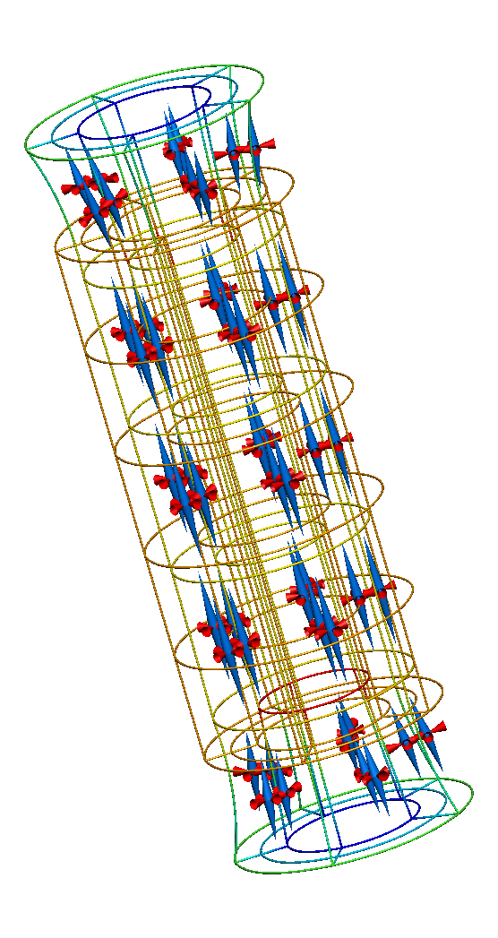
Figure: Results from running this pipe extension simulation. The gold lines show the original, undeformed, cylinder geometry. The coloured lines show the deformed geometry, with the colour varying to show the difference in strain through the wall of the cylinder. The cones represent the three normalised principal strains at material points throughout the tissue volume (red for compression and blue for extension).